This study takes a global view of money. The term “global money” is appearing in recent discussions (Bellofiore 1997) and there is the occasional literature reference to “world money” (Marx 1992: 190). My thesis in this article is that money has a global structure. Stated more precisely, I am contending that (1) the value of money is non-homogeneous throughout the world system (even after exchange rates have been taken into account); that (2) the currencies of low-income countries tend to be undervalued, not overvalued as many economists claim; that (3) the exchange rate system is one of the mechanisms by which high-wage countries extract value from low-wage countries; and that (4) this situation contributes significantly to unequal exchange between periphery and center countries.
These theoretical considerations lead to a new method for quantifying unequal exchange. The Appendix of this study includes World Tables of Unequal Exchange for the year 1995 for 119 countries. These are based on the theory and method developed in this article.
- MONEY AS VALUE AND THE VALUE OF MONEY
It is common knowledge that: (1) money is a measure of value; and (2) money itself has a value. To elaborate the first point: When we buy goods or services, we pay with money (except in barter situations). For example, one pound of bananas is worth x dollars or y rupees in a specific place at a specific time. Or, the entire physical output of a country’s goods and services of a year is measured, not in pounds, tons or number of pieces, but in terms of a single money figure (GDP). In these situations we use money as a measure of value.
To elaborate the second point: We know that money, our measure of value, does not have a constant value. The value of money may change over time (“inflation”) or across space, from one currency zone to another (“exchange rate”). The value of money varies diachronically (longitudinally, over time) and synchronically (cross-nationally, from country to country). Of course, both aspects may be combined.
2. LONGITUDINAL VALUATION OF MONEY
Longitudinal valuation of money is a well-known exercise. The measurement of inflation is in the public eye virtually all the time as, for instance, when the media report the latest inflation rates. These inflation rates are based on scientifically established methods of inflation measurement. Typically, economists define a “basket of goods and services”, measure its price at different points in time and calculate inflation rates from that. While there are disagreements about the finer points of inflation measurement, the longitudinal valuation of money (inflation measurement) is a well-established practice.
3. CROSS-NATIONAL VALUATION OF MONEY
In contrast, the cross-national valuation of money is, partly, well-known and, partly, more obscure. In order to determine the relative value of one currency in comparison with another, two conflicting concepts and measurement procedures exist, namely:
- currency exchange rates between two countries (i.e., the rates at which units of one currency are exchanged for units of another currency; e.g., how many dollars do I get for 100 rupees; how many rupees do 1 get for 100 dollars? etc.); and
- purchasing power parity rates (PPP rates) between two countries (i.e., the ratio of the purchasing power of money in countries A and B; e.g., how much money do I need in order to buy a pair of shoes in country A; and how much money do 1 need in order to buy an equivalent pair of shoes in country B?).
The two concepts differ significantly, though they seem to be similar on the surface. The numbers which one obtains from either method are highly divergent in many situations.
My thesis concerning the global structure of money arises from the difference between these two methods of cross-national valuation of money — namely, exchange rate versus purchasing power parity rate (PPP rate).
4. EXAMPLES
Here are some figures which exemplify the difference that I am talking about (Table 1):
| TABLE 1 – TWO VALUATIONS OF GNP PER CAPITA | |||
| (GNP / capita, 1992 ) | |||
| COUNTRY | METHOD 1: actual exchange rates | METHOD 2: PPP rates (purchasing power parity rates) | COMPARISON |
| US dollars | “international dollars” | ||
| Japan | 28 190 | 20 160 | col. 1 > col. 2 |
| USA | 23 120 | 23 240 | similar values |
| Germany | 23 030 | 20 610 | similar “ |
| UK | 17 790 | 16 730 | similar “ |
| Australia | 17 260 | 17 350 | similar “ |
| Brazil | 2 770 | 5 250 | (factor 1.9) |
| Russia | 2 510 | 6 220 | (factor 2.5) |
| China | 470 | 1 910 | (factor 4.1) |
| India | 310 | 1 210 | (factor 3.9) |
| Bhutan | 62 | 630 | (factor 10.2) |
| Mozambique | 60 | 570 | (factor9.5) |
Source: World Bank. World Development Report 1994, p. 162, p. 220
As the examples in Table 1 show, the value of one country’s money in relation to another country’s money can be calculated using two different methods and expressed in two different rates — exchange rates and PPP rates. For example, the actual exchange rate between Indian rupees and U.S. dollars “shows” that Indian GNP per capita was 310 dollars in 1992. In contrast, scientific measurement of purchasing power parity (PPP) “shows” that Indian GNP per capita was 1210 dollars, i.e. four times as much as shown in terms of exchange rates. OECD countries, however — like the USA, Germany, UK and Australia — have exchange rates to the U.S. dollar that are very similar to the relative purchasing power rates of the currencies.
Which of the two rates (exchange rate versus PPP rate) is the correct one? When we ask the question: “What is the value of rupees in relation to the value of U.S. dollars?”, we obtain two sharply different answers (e.g., “310” and “1210” for GNP per capita in the above). That constitutes a puzzle — not for practitioners, because they use exchange rates, but for scientists. It can be observed that exchange rates are real, in the sense that they are being used by money traders and traders of goods and services. The PPP rate, on the other hand, is scientifically arrived at. Does that mean that PPP rates are not real? Such a conclusion would be untenable. On the contrary, PPP rates are real as well — they are based on carefully established methods of measurement.
The situation is one of a dual standard or a double standard — namely, we have two standards for evaluating the same object. The object to be evaluated is the relationship between money A and money B (the evaluandum) and the two conflicting standards are exchange rate (standard 1) and PPP rate (standard 2). hi order to deal with this discrepancy in a comprehensive manner, we require some theory.
5. TYPES OF THEORY REQUIRED
In order to address the problem as outlined, we require four broad types of theory, namely:
- measurement theory – what is it that we are measuring?
- empirical theory and historical explanation — how can we explain what we see? What causes it? How did it come about?
- theory of value — how can we evaluate what we see? Which standard is the correct one or the best?
- theory of policy (praxis) — what should be done, if anything?
In this study I will not attempt a comprehensive treatment of these issues. Instead, I will focus on two contentions, that: (1) the discrepancies between the two measurement methods are systematic (non-random) and correlate with the global center-periphery structure (empirical claim); and (2) this situation constitutes a form of exploitation (normative claim).
6. HOW PPP RATES ARE CALCULATED
The measurement of PPP exchange rate (purchasing power parity rates) has some similarity with inflation measurement. The method consists of the following: (a) a “basket of goods and services” is defined (as in inflation measurement); (b) prices for this “basket” are collected in the countries around the world — e.g., in country 1 in rubles, in country 2 in rupees, in country 3 in yuan, etc.; (c) the prices for the “basket” in the different countries are compared and permit the calculation of purchasing power parity rates (PPP rates). The World Bank developed and refined this methodology during the past decades to a point where it is as solid as inflation measurement.
The following is a more detailed description, with examples, of the method used for calculating PPP rates. The examples are taken from a handbook by the main authors who developed this method (Kravis, Heston, Summers 1978).
Step (a) — Defining the “Basket”
The first step is to prepare a standardized list (“basket”) of goods and services whose prices are to be compared across countries. The handbook lists 153 categories of goods and services, as follows (Kravis, Heston, Summers 1978: 224-231):
- Rice
- Meal, other cereals
- Bread, rolls
- Biscuits, cakes
- Cereal preparations
- Macaroni, spaghetti
- Fresh beef, veal
- Fresh lamb, mutton
- Fresh poultry
- Other fresh meat
- Frozen, salted meat
- Fresh, frozen fish
- Canned fish
- Fresh milk
- Milk products
- Eggs, egg products
…etc.
- Government expenditures on commodities
These primary items are grouped in various ways, e.g., as follows (Kravis, Heston, Summers 1978: 222):
Consumption
Food
Clothing and footwear
Gross rents and fuels
House furnishings and operations
Medical care
Transport and communications
Recreation and education
Capital formation
Construction
Producers’ durables
Government
Compensation
Commodities
Step (b) — Determine Prices in Local Currency
The handbook does not list the original local prices, but records, for example, how many French francs a Frenchman has to pay in order to buy the same amount of meat that an American gets for one dollar. Here are some examples for the Year 1970, for two countries — France and Colombia (Kravis, Heston, Summers 1978: 175, Table 5.2 and 199, Table 5.18).
| France | Colombia | |
|---|---|---|
| When the American spends one dollar for… |
the Frenchmen pays for the same item… |
the Colombian pays for the same item… |
| Bread and cereals | 4,79 francs | 14,1 pesos |
| Meat | 5,15 francs | 10,9 pesos |
| Fuel and Power | 7,08 francs | 7,0 pesos |
| etc. | etc. | etc. |
Step (c) – Calculate the PPP Rate
These items are further summarized in major groups and for the entire GDP, as follows (Kravis, Heston, Summers 1978: 176,200):
| France | Colombia | ||
|---|---|---|---|
| When the American spends one dollar for… |
the Frenchmen pays for the same item… |
the Colombian pays for the same item… |
|
| Aggregate | |||
| Consumption (items 1-110) |
4,38 francs</td <td8,2 pesos |
||
| Capital Formation (items 111-148) |
4,09 francs | 9,5 pesos | |
| Government (items 149-153) |
4,21 francs | 5,5 pesos | |
| GDP | 4,64 francs | 8,1 pesos | =PPP Rates |
(NOTE: the results for GDP are the purchasing power parity rates between the U.S. dollar and the French franc and between the U.S. dollar and the Colombian peso in 1970)
Step (d) — Calculate the Exchange Rate Deviation
| France | Colombia | Source | |
|---|---|---|---|
| line 1: PPP rate (1970) above |
4,64 francs | 8,1 pesos | step (c) |
| line 2: official exchange rate (1970) | 5,5289 | 18,352 | |
| Kravis,H,S 1978: 8) line 3 = line 2: line 1 exchange rate deviation |
1,23 | 2,26 | Kravis,H,S 1978: 219) |
7. PRACTICAL RELEVANCE OF INVESTIGATION
This investigation may seem abstract, but it has great practical relevance. There is an entire chorus of economists who keep repeating that the exchange rates of poor countries are overvalued. The IMF, in particular, has, over the past two decades and as part of its “Structural Adjustment Programs” (SAPs), forced many countries to devalue their currencies, using the argument that the currency was “overvalued”. This practice has important practical implications for the countries and people affected by SAPs. Furthermore, it reveals two things: (1) the IMF (and the chorus of economists referred to) has a “theory of value” regarding exchange rates. This theory may be largely implicit, but it is there, or else they could not arrive at the evaluative judgment that “exchange rate of country X is overvalued”. And: (2) value theory of exchange rates is of great practical relevance. Whereas most economists agree with the view that the currencies of low-income countries tend to be overvalued, if anything, I claim the opposite, that the currencies of low-income countries tend to be undervalued.
8. EMPIRICAL EVIDENCE: CORRELATION
A look at Table 1 above suggests several observations:
- for the countries of the core of the world system (OECD countries) exchange rates (method 1) and purchasing power rates (method 2) do not differ at all or differ relatively little.
- for the countries of the periphery and semi-periphery of the world system (non-OECD countries) exchange rates (method 1) and purchasing power rates (method 2) yield significantly different results. The difference can be stated in two ways – namely, either: exchange rate values are lower than PPP values, or: the purchasing power value of the country’s currency is greater than the exchange rate value.
- overall, for all countries, it can be observed that the discrepancy tends to be greatest for the poorest countries and least for the richest countries. My Table 1 shows only eleven countries. However, when all countries are examined, the same correlation emerges. Statistical testing of these observations leads to the following results:
- for all countries, there is a statistical correlation between the country’s GNP per capita and the discrepancy between exchange rates and PPP rates. In other words, the poorer the country, the lower will be the exchange rate value of its currency in relation to the PPP value of its currency. Kravis and Lipsey examined this relationship for 34 countries for the year 1975 (including 12 OECD countries and 22 non-OECD countries) and found a very strong relationship between the discrepancy among the two rates and GDP per capita (Kravis and Lipsey 1983: 21). Subsequent studies confirmed the existence of this relationship. My own calculations for 120 countries (based on World Bank data) yield the following observations for the year 1995 (Table 2):
TABLE 2 – CORRELATION
between Currency Value Distortion and GNP per capita, 1995 (n=120 countries)
- Correlation between the “distortion of currency value” and “income level” (GNP/capita): r = – 0.63
- Average distortion factor for 120 countries (standard deviation 1.5): avg d = 2.65
- Maximum distortion factor (Mozambique): max d = 10.1
Minimum (Switzerland, Japan): min d = 0.6 - Classes: average distortion factor for:
- low-income (43 countries): avg d = 4.0
- middle-income (52 countries): avg d = 2.4
- high-income (25 countries): avg d = 0.98
- Average GNP/capita (at exchange rate): US $ 6025
(standard deviation 9408) - Minimum GNP/capita (at exchange rate) (Mozambique): US $ 80
Maximum (at exchange rate) (Switzerland): US $ 40630
Source: World Bank. World Development Report 1997, p. 214-215, Table 1
Note: “GNP per capita” in the correlation is in 1995 US dollars (exchange rate value). The distortion factor is the quotient of GNP per capita “in 1995 international dollars” (i.e. the PPP value), divided by GNP per capita in “1995 US dollars” (i.e. exchange rate value).
9. INTERPRETATION OF THE CORRELATION
In the context of world system theory and related theories (structural theory, imperialism theory), the observed correlation means that a country’s socio-economic status in the world system and the relative value of the country’s money within the world system are related. Topdog countries tend to have “hard” or “strong” currencies (i.e. valuable currencies); underdog countries tend to have “soft” or “weak” currencies (i.e. less valuable currencies). The general power/wealth gradient in the world system can thus be found once more in the value structure of global money.
In terms of causality, it may be asked whether the global power/wealth structure determines the global money structure or vice versa. I assume that both causalities exist. The global power/wealth structure contributes to the global money structure and the global structure of money feeds back into the perpetuation of the global power/wealth structure.
10. VALUE THEORY (NORMATIVE DISCUSSION)
I will now shift from empirical observation to normative reasoning (theory of value). How can we evaluate this situation?
The discussion can be organized around two diametrically opposed evaluative (normative) propositions, namely:
Proposition (1): The exchange rates of low-income countries tend to be overvalued.
Proposition (2): The exchange rates of low-income countries tend to be undervalued.
Let’s examine both propositions.
11. THE OVER-VALUATION ARGUMENT
The over-valuation argument is common and is being used by the IMF, as mentioned earlier. In order to arrive at a verdict of “over-valuation” of a currency, the judging mind must have two things, namely, (a) certain kinds of factual information and (b) a normative standard by which to evaluate the facts; or an evaluation method which implies a normative standard. What normative standard or “yardstick” is being applied by experts who reach the verdict of “overvalued”?
In practice the “Structural Adjustment Programs” of the IMF tend to impose conditions on various countries – conditions which tend to include stipulations about currency. “Typical conditionalities might be: the borrower’s budget or balance of payments deficit must be reduced by x percent within one year;… the currency must be devalued by x percent within six months, etc.” (Brown 1993: 122). There is thus a great concern for balancing the government budget and balancing the balance of payments. The standard by which a currency is evaluated is the balancing of the balance of payments. The connection between this standard and the judgment of “overvaluation” is stated, for example, in the following:
“The currencies of most developing countries are overvalued … When exchange rates are fixed, a surplus demand for foreign currency tends to develop, which must be controlled …”
(Lachmann 1994: 196; my translation.)
The balancing of the balance of payments is thus a major “yardstick” with which the currencies of poor countries are evaluated. (It should be noted that the same yardstick is being applied when the currencies of high-income countries are evaluated.) This may be a valid standard. However, I contend that the following is also a valid standard, even though this argument may seem paradoxical at first.
12. THE UNDER-VALUATION ARGUMENT
When a low-income country (with a structurally distorted currency value, see Table 1) trades with a high-income country, the high-income country gains a quantity of real value which does not show up in any account and the low-income country loses a quantity of real value which does not show up in any account. In colonial times, traders may have exchanged cheap glass beads for valuable ivory. Both sides agreed to the deal. Similarly, a low-income country may make a deal with a high-income country and the deal is balanced in monetary terms at the prevailing exchange rates. However, a quantity of real value is extracted from the low-income country in this deal which does not show up in any account.
The normative standard in this argument is “real value”. I measure “real value” in terms of purchasing power parity (PPP). On this basis, it can be argued that the currencies of the low-income countries tend to be undervalued. Here is an example.
First, let’s eliminate the theoretical possiblity of complete autarky of two countries. In this situation there is no trade and no international money exchange. PPP rates can be measured, but there are no exchange rates. This situation is of no practical interest.
Next, let us examine a situation of balanced trade between country LIC (low-income country) and country HIC (high-income country), with no financial investment across borders, just payments for traded goods and services. (Let’s further assume that LIC has some features of India and HIC has some features of USA. I am using the distortion factor of 3.9 for India from Table 1; the rest in the following is “made up”.)
Here is a 2-country scenario (hypothetical):
[LIC = low-income country
HIC = high-income country]
- LIC has a GDP of 1200 rupees
- HIC has a GDP of 1010 dollars
- The exchange rate of rupee : dollar is 20 : 1
- The two countries trade with each other. The volume of trade between the two countries is 200 rupees = 10 dollars in each direction. In other words, LIC exports goods and services valued as 200 rupees (or 10 dollars) and HIC exports goods and services valued as 10 dollars (or 200 rupees). The trade is balanced. The balance of payments is balanced.
Now let us examine the implication of the distortion factor. The distortion factor in crossnational currency valuation is 3.9 (from Table 1). This means that the purchasing power rate (PPP rate) between LIC’s rupee and HIC’s dollar is not 20 : 1 but, rather, 20/3.9 : 1 = 5.13 : 1. I am rounding this off to 5 : 1 .
When we assume that the PPP rate reflects the true value of the currency, then it can be observed that:
- from LIC’s point of vicw: LIC exported goods and services worth 200 rupees. In exchange, LIC imported goods and services worth 200 / 20 = 10 dollars at exchange rate. However, LIC would have imported 200 / 5 = 40 dollars worth at PPP rate. The monetary distortion factor had the effect that LIC lost 40 – 10 = 30 dollars worth of imports due to the distortion factor. This loss of 30 dollars, at PPP rate, corresponds to 150 rupees.
- from HIC’s point ofview: HIC exported goods and services worth 10 dollars. In exchange, HIC imported goods and services worth 10 * 20 = 200 rupees at exchange rate. However, HIC would have imported 10 * 5 = 50 rupees worth at PPP rate. The monetary distortion factor had the effect that HIC gained 200 – 50 = 150 rupees worth of imports due to the distortion factor. This gain of 150 rupees, at PPP rate, corresponds to 30 dollars.
- Summary: Due to the monetary distortion factor between the two currencics, LIC lost 150 rupees worth of import value; HIC gained 30 dollars worth of import value. These losses and gains of value do not show up in the accounts, because the value of money is itself structurally deformed. The trade is formally balanced.
As a percent of GDP, the gains and losses are, as follows: LIC has an “invisible loss” (unrecorded loss) of 150 rupees. With a GDP of 1200 rupees, the invisible loss of value is 150/1200 = 12.5% of GDP. HIC has an “invisible gain” (unrecorded gain) of 30 dollars. With a GDP of 1010 dollars, the invisible gain of value is 30/1010 = 3.0% of GDP.
Based on this reasoning, I conclude that the currency values of low-income countries tend to be undervalued. The effect is exploitative. The core countries appear to extract a large amount of value from the periphery countries through the clever monetary device called exchange rate system. Babones (1998) has recently made a parallel observation with respect to global center-periphery relations, namely that: “Surplus value is not extracted solely through coercion, but also through the working of financial markets.” (He is referring to credit markets.)
13. RECENT LITERATURE ON UNDERVALUATION
Undervaluation of currencies has drawn some attention in the 1990s. In a recent study, Havlik argues for currency undervaluation, stating with reference to countries in Central and Eastern Europe that “undervaluation is needed in order to overcome institutional, structural and quality deficiencies” (Havlik 1996). Yotopoulos (1996), however, argues against currency undervaluation in a book that combines theory, statistical-empirical research and case studies. He uses purchasing power parity (PPP) data from World Bank sources, compares them with nominal exchange rates (NER) and calculates an exchange rate deviation index (ERD) for all countries (Yotopoulos 1996: 97-100). The study investigates the relationship between currency valuation and economic growth. His observations agree with mine in two important points — namely, Yotopoulos writes: (1) “free currency markets … have an inherent distortion” (Yotopoulos 1996: ii) and (2) with reference to low- and middle-income countries: There is “undervaluation of the NER [sc. nominal exchange rate]… Conventional wisdom, on the contrary, sees the problem as NER overvaluation …”(Yotopoulos 1996: 8. Emphasis original)
14. THE QUANTIFICATION OF UNEQUAL EXCHANGE
The availability of PPP data and the possibility of calculating an exchange rate deviation index (variable “d” in Table 2 above; or “ERD” in Yotopoulos 1996) opens up an intriguing new way of quantifying the degree of “unequal exchange” (losses and gains from unfair center-periphery trade).
In Emmanuel’s theory the concept of “unequal exchange” is the grand dependent variable. In his words: “…unequal exchange is the proportion between equilibrium prices that is established through the equalization of profits between regions in which the rate of surplus value is ‘institutionally’ different…” (Emmanuel 1972: 64).
This is a theoretical definition and not an operational definition. How unequal is the exchange? How much value is unfairly transferred from the periphery to the center?
Emmanuel did not give any precise figures, and this measurement problem was still relatively unresolved in 1987, when Raffer reviewed the state of the art with respect to the measurement of unequal exchange (Raffer 1987: chapter 11). However, Emmanuel gave a sense of magnitudes involved when he wrote that the:
“loss [sc. resulting from unequal exchange]… is enormous in relation to the poverty of the underdeveloped countries while being far from negligible in relation to the wealth of the advanced countries.” (Emmanuel 1972: 265)
Some authors provided estimates for individual countries. Gibson (1980) estimated a loss for Peru in 1969 in its trade with USA as 38% of its exports to the USA (sec, Raffer 1987: 94). Webber and Foot (1984) estimated for the Philippines in 1961 that Philippine exports would have amounted to 5.269 billion pesos, if valued at Canadian wages and prices, instead of the actual 1.129 billion pesos (see, Raffer 1987: 95).
A worldwide estimate is available from Samir Amin. Amin estimated the loss incurred by developing countries for the year 1966 as being $22 billion. That corresponds to a loss of 15% of GDP for the developing countries and to a gain of 1.5% of GDP for the advanced countries. (Amin 1976: 143-144 and Raffcr 1987: 93-94)
One expert on unequal exchange, Raffer, stated in 1987 that “precise statistical methods of measuring [sc. unequal exchange] are still lacking.” (Raffer 1987: 194) That was the state of affairs in the late 1980’s. In the meantime, a new type of data has become widely available, namely, the World Bank’s PPP data which are now available for a majority of countries. In combination with a structural view of global money, these data can be used for estimating the degree of unequal exchange. The following calculations for 1993 are illustrative of such a possibility.
The proposed estimation method is, as follows: (a) calculate the distortion factor d (see above. Tables 1 and 2, or, as Yotopoulos calls it, the ERD — exchange rate deviation index); and (b) apply it to the volume of trade, giving (c) the loss or gain due to unequal exchange, according to the formula:
T = d*X – X
where:
T = magnitude of unrecorded transfer (loss or gain) due to unequal exchange
X = volume of exports from a low-wage country to high-wage countries, and d = the distortion factor (i.e. the deviation of the nominal exchange rate from the PPP rate, also known as ERD)
The formula means, in words, that the unrecorded transfer (T) resulting from unequal exchange is equal to the difference between the fair value of the export (d * X) and theunfair (actual) value of the export (X). For low-wage countries this magnitude T is a loss. For high-wage countries the same magnitude T is a gain.
Hypothetical example: A low-income country has exports to a high-wage country of X = $1000 and a distortion factor of d = 2.65 (which is average, sec Table 2). Instead of earning $1000 from exports, the country could have earned 2.65 * $1000 = $2650. The difference 2650 (fair value) – 1000 (unfair value) = $1650 is the amount of unrecorded value lost by the low-wage country (and gained by the high-wage country) due to unequal exchange. When Emmanuel first presented his ideas (1962 and 1969/72), PPP data were not available, so that this kind of quantification of the effects of unequal exchange was not possible at the time.
15. ESTIMATES OF UNEQUAL EXCHANGE FOR 1993
This estimation method can be applied to export data for 1993. The export streams between center and periphery of the world arc shown in Table 3:
Table 3. World Export Flows, 1993
| U.S. dollars trillions (at exchange rates) |
||
|---|---|---|
| TO: OECD |
TO: non-OECD |
|
| FROM: OECD | 1,84 | 0,70 |
| FROM: non-OECD | 0,64 | 0,46 |
| WORLD, total exports = 3,70 US $ trillions | ||
U.S. dollars trillions (at exchange rates)
NOTE(a): non-OECD = “developing countries” + Eastern Europe and former USSR. Source: United Nations. Yearbook of International Trade Statistics 1995, Vol. 2, Special Table B, page S 22
The figure to watch in Table 3 is “0.64”. This represents the exports from the periphery (all non-OECD countries) to the center of the world system (OECD countries) and shows periphery-to-center exports as US $ 0.64 trillion (or, $640 billion). When we value this volume of exports in terms of PPP rates, then the distortion factor of 2.65 (from above) can be applied as a first approximation. Given this preliminary assumption, the fair value of the export flow of US $0.64 trillion can be valued as 0.64 * 2.65 = 1.7 trillions of PPP dollars. If this is the fair value of the exports from low- and middle-income countries to high-income countries, then the amount of income lost by low-and middle-income countries in 1993, due to unequal exchange, may be estimated as:
d*X – X = T
(fair value) less (unfair value) = (loss due to unequal exchange) or,
1.7 – 0.64 = 1.06
In other words, in 1993 the loss incurred by low- and middle-income countries due to unequal exchange may have been 1.06 trillion of PPP dollars. At the same time, this is the estimated gain for OECD countries.
How does this figure compare with global GDP and the GDPs of low- and high-income countries? The GDP figures for the world in 1993 arc given in Table 4:
Table 4 – World GDP, 1993
| (US dollars trillions) |
|
|---|---|
| COUNTRY CLASS | |
| High-income | 18,6 |
| Low- and middle-income | 5,0 |
| WORLD | 23,6 |
| Source: World Bank, World Tables 1995, p. 29 | |
Using Table 4 data we can calculate the unrecorded transfer (T) of $1.06 trillion, which results from unequal exchange, as a percent of GDP, namely:
- OECD countries: 1.06 /18.6 = 5.7 % of GDP (of OECD)
- non-OECD countries: 1.06 / 5.0 = 21.2 % of GDP (of non-OECD)
16. COMPARISON OF ESTIMATES OF UNEQUAL EXCHANGE
A comparison of Amin’s estimates of the degree of unequal exchange with my estimates yields the following summary (Table 5):
Table 5 – Comparison of Estimates of Unequal Exchange
| For Year |
For Unit of analysis |
Estimate In current US dollars |
Estimate as a percent of GDP of |
||
|---|---|---|---|---|---|
| LIC(a) | HIC(a) | ||||
| Amin | 1966 | developing countries |
22 billion | -15% | +1,5% |
| Köhler | 1993 | non-OECD countries |
1,06 trillion | -21% | +5,7% |
NOTE (a): LIC = low- and middle-income countries; HIC = high-income countries Sources: see text above
Table 5 shows similarities and discrepancies in the estimated percentages. Whether global exploitation increased between 1966 and 1993, as the table seems to suggest, is difficult to answer since Amin’s and my estimates are based on two different methods. This problem requires further research.
However, it can be observed that both methods lead to roughly comparable magnitudes. Furthermore, the figures are consistent with Emmanuel’s non-quantitative statement – namely, that the “loss [sc. resulting from unequal exchange],..is enormous in relation to the poverty of the underdeveloped countries while being far from negligible in relation to the wealth of the advanced countries.” (Emmanuel 1972: 265)
17. IMPLICATIONS FOR THE THEORY OF UNEQUAL EXCHANGE
In the history of science new instruments and new types of data have, on numerous occasions, led to innovations in theory-e.g., the invention of the telescope in astronomy; the invention of the microscope in biology; the development of computer-based timeseries analysis in economics, etc. Similarly, the availability of PPP data, which were not available in the 1960’s and 1970’s and not fully available in the 1980’s, are now adding new insights to the theory of unequal exchange. The subtitle of Emmanuel’s book “Unequal Exchange” is “A Study of the Imperialism of Trade”, where trade refers to commodity trade, not currency trade. With the help of now-available PPP data, it becomes increasingly apparent that the element of unfairness or exploitation in the notion of “unequal exchange” is not only a matter of unequal commodity exchange, but also a matter of unequal currency exchange, both being intricately linked.
Emmanuel’s theory of unequal exchange includes the following views:
- Trade between low-income and high-income countries (periphery and center of the world system) is unequal, meaning: unfair, biased against the low-income countries.
- Wages in low-income countries are undervalued in relation to wages in high-income countries.
- Export prices of exports from low-income countries are undervalued in relation to the export prices of high-income countries.
- There is a relationship between the undervaluation of labour and the undervaluation of exports of low-income countries. Emmanuel stresses that: “… inequality of wages as such, all other things being equal, is alone the cause of the inequality of exchange” (Emmanuel 1972: 61) and refers to wages as “the independent variable of the system” (Emmanuel 1972: 64).
What causes the inequality of wages between high-wage and low-wage countries? Here Emmanuel discusses various possible influences — physiological wage, historical wage, market wage, equilibrium wage, moral element, trade-union factor, wage zones and so on. (Emmanuel 1972: 109-122) Generally, the problem is seen as an “institutional” problem.
In terms of causal modelling, Emmanuel constructs a causal sequence from antecedent factors A1, A2, A3 etc. (called “determinants of wages”), which cause “inequality of wages” (X), which in turn is causing “unequal exchange of commodities” (Y). That is:
A → X → Y
An alternative causal view, based on a structural view of global money, is that the “undervaluation of a country’s currency” has two simultaneous valuation effects as a consequence of the distorted structure of global money (M): (X) it leads to an undervaluation of labour in the low-income country relative to labour of high-income countries; and (Y) it leads to an undervaluation of the exports of the low-income country relative to the exports of high-income countries. That is:
→X
M
→ Y
Seen this way, the unfairness of commodity trade between low-wage and high-wage countries (“unequal exchange” in Emmanuel’s sense) is, in part, caused by the structure of global money (“unequal exchange” in the sense of “unequal exchange rates”). The distortion of global money and of the exchange rate system is shaped by the historically grown structure of the world-system (center-periphery, imperialism, “global apartheid” (Kohler 1978,1995)) and ideologically supported by neoclassical international economic theory (favouring free/unregulated currency markets).
18. IMPLICATIONS FOR PRAXIS
Unequal exchange theory supports an advocacy of labour struggle with the objective of raising the wages of workers in peripheral countries and/or an advocacy of global socialism, for example, along the lines of Amin’s socialist polycentrism (Amin 1994). The structural view of global money suggests an additional strategy, which may be combined with the above strategies or pursued on its own, namely: a reform of the global exchange rate system in the direction of purchasing power parity (PPP) rates. Such a reform would raise the wages of low-income countries relative to high-income countries, as fought for by Emmanuel and others; it would improve the terms of trade for low-income countries, as fought for by Prcbisch and others; and it would significantly reduce unequal exchange.
How much each low- or middle-income country could gain from such a global monetary reform — and how much it is presently losing due to unequal exchange, can be seen from the World Tables of Unequal Exchange which arc presented in the Appendix below. These tables arc based on the theory and method developed in this article.
19. REFERENCES
Amin, S. (1976) Unequal Development. New York, EISA: Monthly Review Press [translated from the 1973 French original]
Amin, S. (1994) “The Future of Global Polarization”, Review (Fernand Braudel Center, USA), XVII, 3 (Summer), p. 337-347
Babones, S. (1998) “A Credit-Market Theory of Surplus Value”, forthcoming.
See, memorandum, wsn mail archive, 08 Dec 1997,
http://csf.colorado.edu/maiPwsn/currenfr0331.html
Bellofiore, R. (1997) memorandum, concerning a recent conference in Italy with a section on “Global Money, Capital Restructuring and the Changing Pattern of Production”, pkt mail archive, 13 Nov 1997, http://csf.colorado.edu/mail/pkfrnov97
Brown, R.S. (1993) “The IMF and the World Bank in the New World Order,” in: P. Bennis and M. Moushabeck, eds., Altered States: A Reader in the New World Order. New York, USA: Olive Branch Press
Emmanuel, A. (1972) Unequal Exchange: A Study of the Imperialism of Trade. New York, USA: Monthly Review Press [translated from the 1969 French original]
Havlik, P. (1996) “Exchange Rates, Competitiveness and Labour Costs in Central and Eastern Europe,” WIIW Research Report No. 231 (October)
Abstract available at: http://www.wiiw.ac.at/summ231 .html
Kohler, G. (1978) “Global Apartheid”, Alternatives (Institute for World Order / World Policy Institute, USA), 4, no. 2 (October), p. 263-275
_ (1995) “The Three Meanings of Global Apartheid: Empirical, Normative, Existential”, Alternatives, 20 (1995), p. 403-423
Kravis, I.B., A. Heston and R. Summers (1978) International Comparisons of Real Product and Purchasing Power. Baltimore, USA: Johns Hopkins University Press.
Kravis, I B. and R E. Lipsey (1983) “Toward an Explanation of National Price Levels,” Princeton Studies in International Finance, No.52, November 1983 (Princeton University, USA. Department of Economics.)
Lachmann, W. (1994) Entwickhmgspolitik. Munchen, Germany: Oldenbourg Verlag
Marx, K. (1992) Capital, vol. 2. Penguin edition 1978 [reprinted 1992]
Raffer, K. (1987) Unequal Exchange and the Evolution of the World System. London, England: MacMillan Press
United Nations (1995) Yearbook of International Trade Statistics 1995, Vol. 2
World Bank (1995) World Tables 1995
_ (1994) World Development Report 1994
_ (1997) World Development Report 1997
Yotopoulos, P.A. (1996) Exchange Rate Parity for Trade and Development: Theory, tests, and case studies. Cambridge, England: Cambridge University Press
APPENDIX WORLD TABLES OF UNEQUAL EXCHANGE
1995, 119 countries
21. INTRODUCTION
The statistical tables below present quantitative estimates of unequal exchange for 119 countries. The tables are based on the theory and method developed in the main body of the article. The calculations are based on export/import data and the exchange rate deviation index. Losses or gains from unequal exchange are calculated as the difference between a “fair value” of exports/imports and the “actual (unfair) value” of exports/imports. The estimation formula is:
T = d*X – X
where
d = the exchange rate deviation index (also designated as “ERD” in the literature) X = the volume of exports from a low- or middle-income country to high-income countries (valued at the actual exchange rate)
T = the unrecorded transfer of value (gain or loss) resulting from unequal exchange
In the tables (below), this formula is applied to the data for 119 countries for the year 1995.
22. HOW TO READ THE TABLES
Table 1 presents the step-by-step calculations. Countries are arranged in alphabetical order and in two groups — first, non-OECD countries and, secondly, OECD countries. The losses or gains from unequal exchange are shown at the right-hand side (in terms of U.S. dollars and as a percent of the country’s GNP).
Table 2 presents the losses and gains (same as in Table 1), sorted by dollar volume.
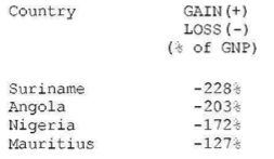
Table 3 presents the losses and gains (same as in Table 1), sorted by percent of GNP.
The tables are followed by a brief discussion and further methodological details.
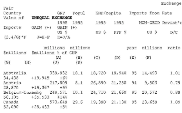
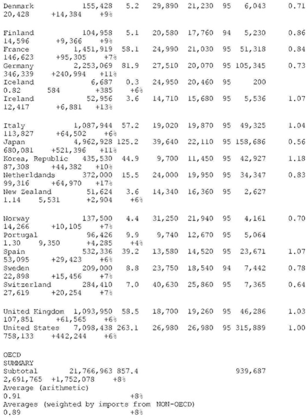
23. THE WORLD TABLES
Table A-1 – WORLD TABLE OF UNEQUAL EXCHANGE 1995
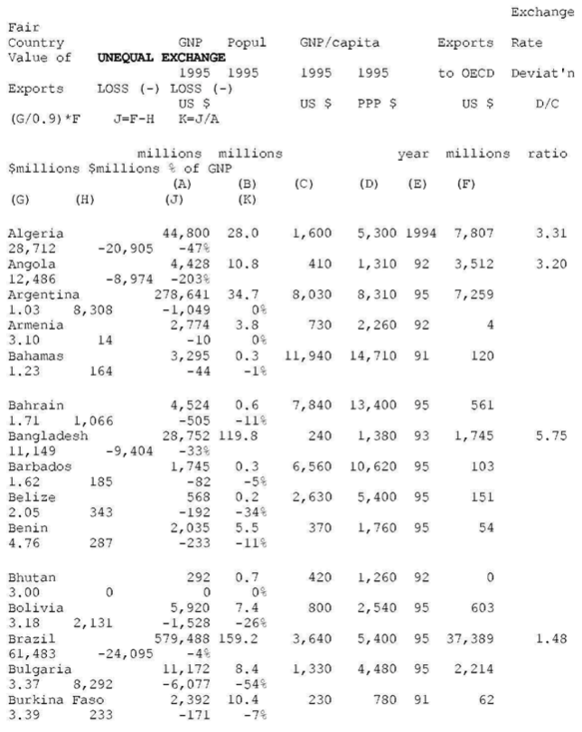
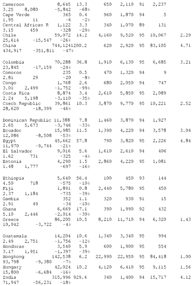
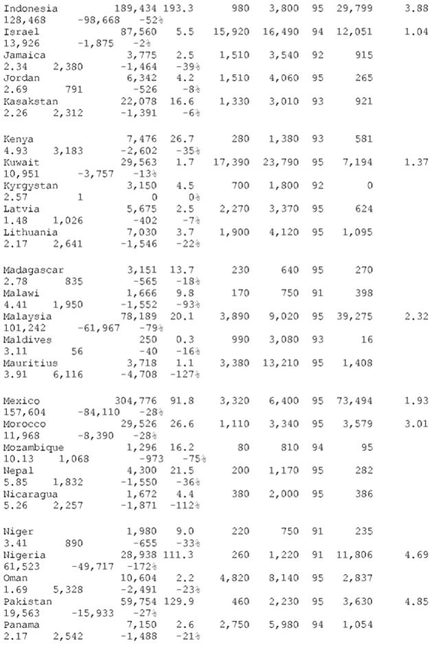
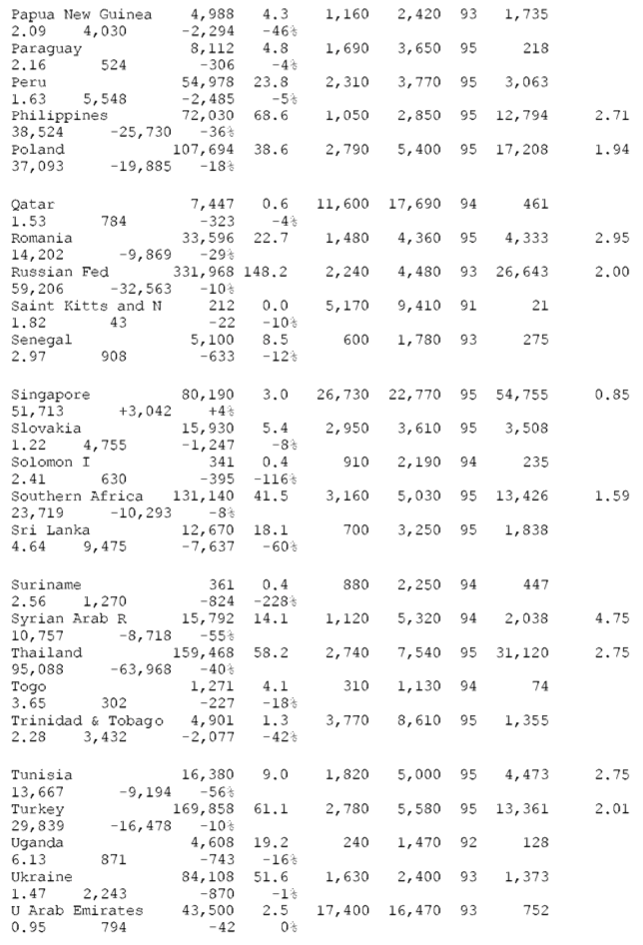
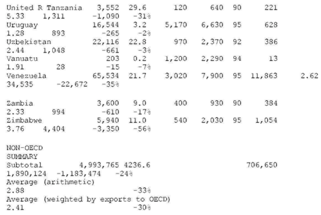
OECD countries (N=22)
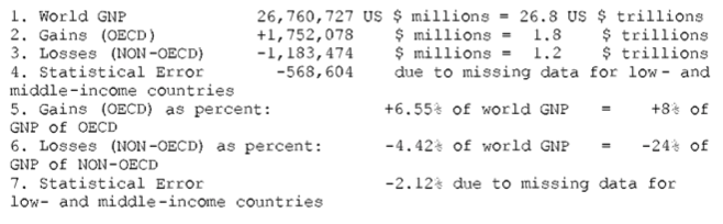
WORLD SUMMARY ON UNEQUAL EXCHANGE 1995 (N = 119 countries)
SOURCES
- for columns B, C, D (population, GNP per capita, PPP values, list of OECD countries): World Bank. World Development Report 1997, p.214-215 (Table 1), p.248 (Table 1a), p.265 (Table 1)
- for columns E, F (year and volume of exports or imports):
United Nations. International Trade Statistics Yearbook 1995, Vol. 1. For each country, Table 3 (“Trade by Principal Countries of Production and last Consignment”) was used.
Aggregation: “NON-OECD” = “World”[from source] – “OECD”.
“OECD” = [from source:]”Northcrn America” + “EEC” + “EFT A” + “other Europe” + “Oceania” + “Japan” + “Korea, Republic of”
CALCULATIONS
col. A = B * C
col. B, C, D, E: none
col. F: see “SOURCES #2”
col. G = D / C (= d, = exchange rate deviation)
col. H: two formulae—(1) NON-OECD, fair value of exports to
OECD:(d/0.9)*exports=(colG/0.9)* col. F ( 0.9 is the average exchange rate deviation for the block of OECD countries, see above)–(2) OECD, fair value of imports from NON-OECD:(2,4/d) *imports=(2.4/G)* col. F ( 2.4 is the average exchange rate deviation for the block of NON-OECD countries, see above)
col. J — for losses: J= F – H— for gains: J = H – F
col K = J / A as a percent
End Table A-1
TABLE A-2–WORLD TABLE OF UNEQUAL EXCHANGE 1995: SORTED BY VOLUME
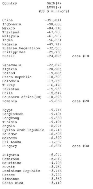
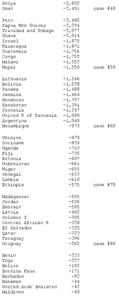
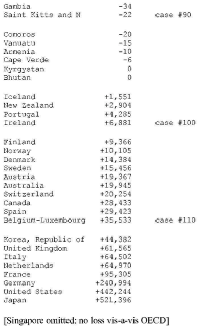
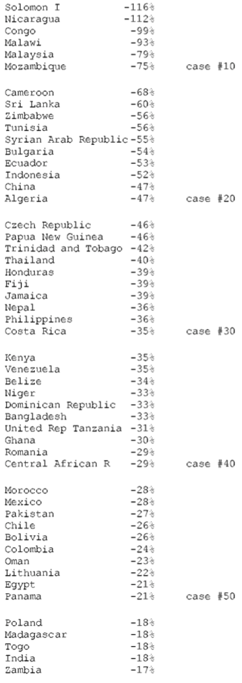
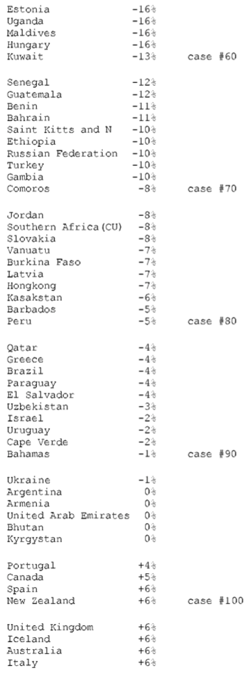
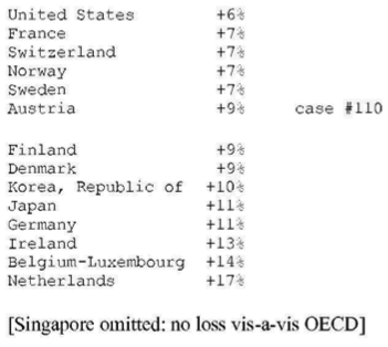
TABLE A-3 – WORLD TABLE OF UNEQUAL EXCHANGE 1995: SORTED BY PERCENTAGE
24. SELECTED FINDINGS FOR THE YEAR 1995
(a) The average exchange rate deviation (from PPP = 1.0 = value of U.S. dollar) for the block of non-OECD countries is d = 2.4 and for the block of OECD countries d = 0.9.
(b) The aggregate gain by OECD countries due to unequal exchange is $1.75 trillion. The aggregate loss by non-OECD countries is the same as the gain by OECD countries. However, the table shows only an aggregate loss of $1.18 trillion for all non-OECD countries. The discrepancy is due to missing data for non-OECD countries.
(c) In percentage terms the gains and losses are as follows: 6.6% of world GNP is transferred from low- and middle-income countries to high-income countries due to unequal exchange (unrecorded transfer of value). This is the equivalent of +8% of OECD GNP and -24% of non-OECD GNP (in the aggregate ) or -33% on average of the GNPs of individual non-OECD countries.
(d) The three countries with the highest volume losses arc: China (-0.35 trillion or 351 billion U.S. dollars), Indonesia (-0.1 trillion or 99 billion dollars), and Mexico (-0.08 trillion or 84 billion dollars). The three countries with the highest volume gains are Japan (+0.5 trillion of or 521 billion dollars), United States (+0.4 trillion or 442 billion dollars), and Germany (+0.24 trillion or 241 billion dollars).
(e) The three countries with the highest percentage losses are Suriname (-228% in relation to GNP), Angola (-203%), and Nigeria (-172%). The three countries with the highest percentage gains are Netherlands ( +17% in relation to GNP), Belgium-Luxembourg ( +14%), and Ireland ( +13%).
25. DISCUSSION
25.1. ARE THE NUMBERS VALID?
There are several reasons why these calculations may be valid:
- The numbers are based on data from reputable sources (United Nations and World Bank);
- The numbers are broadly compatible with prior estimates of unequal exchange losses and gains — e.g., Samir Amin estimated for 1966 an aggregate loss by developing countries of 22 billion U.S. dollars (1966 value), corresponding to 15% of the GNP of developing countries (Amin 1976: 143-144 and Raffer 1987: 93-94);
- The numbers are consistent with notions of unequal exchange, unequal development and unequal terms of trade as discussed in a large body of theoretical literature;
- The numbers give a statistical view of the world which corresponds to the experience of the people of low- and middle-income countries;
- The numbers appear to have some explanatory power with respect to understanding the massive global polarization of incomes which has been observed and criticized by many observers.
25.2. PRACTICAL VALUE
These tables may be of practical value for low- and middle-income countries. The dollar losses from unequal exchange can be used as dollar claims against the world system and the high-income countries.
25.3. DO LOW- AND MIDDLE-INCOME COUNTRIES LOVE TO BE EXPLOITED?
Most existing trade theory argues that countries would not engage in international trade if they did not gain from doing so. Furthermore, earlier leftist calls for disengagement from the international capitalist trading system were more and more ignored by low- and middle-income countries. Even the relative isolation of present-day Cuba from world trade is involuntary. Can it not be concluded that “no trade” is bad and “trade” is good for low- and middle-income countries?
Without going into a major theoretical argument at the conclusion of this study, I would like to offer the following observation, based on the statistical tables above. The amount of unequal exchange loss by a country is a function of two variables in the formula, namely, exchange rate deviation (d) and volume of trade with high-income countries (X). If a country has no trade with OECD, it cannot be exploited by OECD. On the down side, this country cannot “make money” by trading with OECD either. If a poor country engages in significant trade with the rich countries, it has a chance to “make money” (gains from trade). If its currency has a fair value, then this trade is fair and the gains are fair. If its currency does not have fair value, however– that is, if it has a high exchange rate deviation (d) — then this country experiences gains from trade and exploitation through trade at the same time. The situation is comparable to that of a worker vis-a-vis an exploitative employer, as captured in the following table of options and outcomes (Table 4):
Table A-4. Options/Outcomes
| OPTIONS | OUTCOMES | ||
| worker-employer | poor country-rich country | ||
| option 3 | good job | fair trade | make good money, happy and satisfied |
| option 2 | bad job, underpaid overworked | unequal exchange, undervalued unfair trade | make some money, have an income at exploitation rates |
| option 1 | no job | no trade | make no money, starve |
As Table 4 indicates, if the choice is between “no job” and a “bad job”, the worker gains by taking the bad job. Similarly, if a country has a choice between “no trade” and “unfair trade”, the country gains by engaging in unfair trade. However, a good job or fair trade are immensely preferable to a bad job or unfair trade. In this sense, it is possible to “gain from trade” and be “exploited through trade” at the same time. A country may have little choice between options 1 and 2 but may want to fight for option 3.
26. FURTHER METHODOLOGICAL DETAILS CONCERNING THE WORLD TABLES
(a) Exclusion of countries: Countries which are not shown in the tables are missing due to missing data. For these countries either export data or PPP data or both were missing in my sources.
Luxembourg is lumped together with Belgium because the export/import data were given that way in the source. (The GNP-related data are for Belgium.)
(b) Two calculation models:
There are two calculation models, one for non-OECD countries and one for OECD countries. Both use the same formula (see above) with two slight variations.
MODEL 1 for non-OECD countries:
Here I measure the export flow from each individual non-OECD country to the block of OECD countries. Since the exchange rate deviation for the block of OECD countries is d = 0.9 (i.e. deviation from the U.S. dollar), the exchange rate deviation between the individual non-OECD country and the block of OECD countries is not d(to OECD) = d/1.0 since the d calculated from the source gives the deviation to the U.S. dollar. Instead, the deviation to the block of OECD is d(to OECD) = d/0.9.
MODEL 2 for OECD countries:
Here I measure the import flow from the block of non-OECD countries to each individual OECD country. Since the exchange rate deviation for the block of non-OECD countries is d = 2.4 (i.e. deviation from the U.S. dollar), the exchange rate deviation between the individual OECD country and the block of non-OECD countries is not d(to non-OECD) = 1.0/d since the d calculated from source gives the deviation to the U.S. dollar. Instead, the deviation to the block of non-OECD is d(to non-OECD) = 2.4/d.
(c) Statistical discrepancies and errors:
There are three statistical discrepancies and errors of which the reader should be aware:
- The world GNP shown in the table is not exactly the same as the world GNP which may be shown elsewhere. This is due to the fact that numerous non-OECD countries are missing in the table, including major oil producers like Saudi Arabia, Iran and Iraq. However, I did not correct that in order to keep the numbers in the table consistent with each other. (The same applies to world population.)
- The total of exports from non-OECD to OECD shown in the table is not the same as the total of imports by OECD from non-OECD. This is a result of a large number of missing non-OECD countries. As the data for the OECD countries are complete, the larger of the two totals (namely, total imports by OECD from non-OECD) is the correct figure and the total of exports from non-OECD to OECD is understated.
- The total losses shown for non-OECD countries arc not the same as the total gains by OECD countries. This is a consequence of missing data for non-OECD countries. As the data for OECD countries are complete, the total gains by OECD countries is the correct total for global exploitation due to unequal exchange. The total of losses by non-OECD countries is understated. However, the losses for individual non-OECD countries shown in the table are correct for each individual country.
The article was originally published in Journal of World-Systems Research, vol. 4, pp 145-168
This article has been published with the permission of the author and the copyright holder. The usual Creative Commons license does not apply.